Quantum States, Collapse, and the Quantum Mystery
A clear and thought - provoking investigation of how observation shapes the reality of quantum states.

Hi, I’m Ayo! I’m a first-year student majoring in Computer Science and minoring in Physics. I love helping others see the exciting aspects of quantum computing and AI. When I’m not studying or writing about technology, you’ll likely find me watching shows, catching up on videos, or playing basketball or pickleball. Fun fact: I’ve never broken a bone!
Revisiting Classical Systems: The Foundation of Probability
Last week, we went into great detail about the fundamentals of general, multi-state classical systems, grounding their mathematical representation in the spirit of linear algebra and basis vectors. To ease a smoother transition into quantum concepts, we introduced the concept of Dirac notation, which is a convenient and shorthand way of representing the basis vectors corresponding to distinct states.
Before we move on to quantum computing, let us reanalyze the Lighdie analogy from a new angle.
Lighdie’s Classical Library Analogy
In our original analogy, Lighdie was faced with the daunting task of brushing aside her teenage angst by selecting a book from the existing catalog of quantum books on Shor’s Algorithm (SA), Grover's Algorithm (GA), and the Phase Kick Back technique (PKB). Recall that Lighdie’s probability distribution $(0.3, 0.6, 0.1)$of selecting the $SA$, $GA$, and \(PKB \\\), respectively, led to the following classical state:
$$\psi = 0.3 \ket{PKB} + 0.6 \ket{SA} + 0.1 \ket{GA}$$
Where \(\ket{SA}, \text{and } \ket{GA}\)are the Dirac-notation equivalent of the following unit vectors
$$\quad |PKB \rangle = \pmatrix{ 1 \\ 0 \\ 0},\quad |SA\rangle = \pmatrix{ 0 \\ 1 \\ 0},\quad |GA \rangle = \pmatrix{ 0 \\ 0 \\ 1}$$
, and \(\psi\) is the classical system.
Understanding Post-Measurement Determinism
Dirac ket notation is concise and elegant, but it falls short in explaining the underlying meaning behind the obscure 1s and 0s in each basis vector. To bridge this conceptual gap, we now introduce the idea of post-measurement determinism by revisiting the second rule of Lighdie’s angsty library spree:
Every time Lighdie decides to select a book from the existing catalog, her rays of light destroy the other existing books in the catalog.
If taken at face value, the rule seems absurd — clearly the product of a sleep-deprived individual (don’t worry, guys, I get plenty of sleep!). However, we quickly realize that this statement reflects the fact that classical systems become deterministic once measured.
In other words, before Lighdie makes a selection, \(\psi\) is uncertain and unmeasured. After a selection is made, the system \(\psi\) collapses to that choice with a probability of $1$, which is reflected. For example, if Lighdie selects the book (SA), then \(\psi\) collapses to the state:
$$\ket{SA} = \pmatrix{ 0 \\ 1 \\ 0}$$
Where the 1 represents that Lighdie has made her selection to SA with absolute certainty.
Similarly, if Lighdie selects the book PKB, then \(\\psi\) collapses to the state
$$\ket{PKB} = \pmatrix{1 \\ 0 \\ 0}$$
with absolute certainty.
The Mathematics of Classical Probability
Keep in mind that there is an infinite number of classical systems one can construct. These classical states can represent anything tangible, from fruits to cards. For the sake of generality, if we take \(\mathbf{n}\) general classical states \(c_1, c_2, \dots, c_n\) with corresponding probabilities \(p_1, p_2, \dots, p_n\), then we can describe an arbitrarily large classical system \(\phi\) such that:
$$\phi = p_1\ket{c_1} + p_2\ket{c_2} + \dots + p_n\ket{c_n} = \sum_{i=1}^n p_i \ket{c_i}$$
Notice that the represent all valid outcomes in the system \(\phi\), which means that:
$$\sum_{i=1}^{n} p_i = 1, \text{all p_i are non-negative}$$
Now that we have constructed a complete mathematical description of any classical system, we are ready to investigate the peculiarities of quantum randomness.
Introducing Quantum Randomness
We will begin by repurposing our previous analogy to explain quantum randomness or superposition.
Consider an alternate dimension to Lighdie’s universe, where an individual named Mighty resides. Mighty is also an extremely angsty teen who is motivated to visit the library, where he discovers a peculiar book adorned by three unique titles — Shor’s Algorithm, Grover’s Algorithm, and Phase Kick Back technique.
Mighty and the mScanner: A New Dimension of Uncertainty
Curious and suspicious of the front cover, Mighty flips to the back cover, where he finds an even stranger description:
When you scan this book, you can expect:
A γ² chance of receiving Shor’s Algorithm book,
A β² chance of receiving Grover’s Algorithm,
A α² chance of eceiving the Phase Kick Back book.
Utterly flabbergasted by this blurb, Mighty decides to seek assistance from the librarian. She simply tells him,
“That’s how quantum books work — you don’t know which book you will receive till you measure it.”
Reluctantly, Mighty scans the book using a mysterious mScanner and is shocked when it morphs into a red 500-page text on the Phase Kick Back Algorithm. He quickly checks his receipt, which reads:
The Quantum Receipt
Quantum Book:
Original State: \(\ket{book} = \alpha \ket{PKB} + \beta \ket{SA} + \gamma \ket{GA}\)
Amplitudes: \(\alpha, \beta, \gamma\)
Possible Books: \(\ket{PKB}, \ket{SA}, \ket{GA}\)
Measuring Device: mScanner
Result: \(\ket{PKB}\)
This receipt captures the true meaning of quantum states. The original state of Mighty’s mysterious book was in a superposition of SA, GA, and PKB. In other words, when Mighty first encountered the book, it was truly all of these three books at the same time.
In particular, the state is formally:
$$\alpha \ket{PKB} + \beta \ket{SA} + \gamma \ket{GA}$$
where the coefficients \(\alpha, \beta , \gamma \) are called amplitudes, whose square magnitudes give the probability of observing each outcome:
$$P(|PKB\rangle) = |\alpha|^2, \quad P(|SA\rangle) = |\beta|^2, \quad P(|GA\rangle) = |\gamma|^2$$
Similar to Lighdie’s classical randomness, applying the mScanner measurement device to the quantum book collapsed it into one definite state. Unlike the classical version, amplitudes encode the system's randomness instead of direct probabilities.
Looking Ahead
That concludes this week's blog and the final part of my all-immersive quantum computing introduction!
In the following weeks, we will be exploring the strange mathematical rules governing amplitudes and explaining why quantum states must always be normalized.